Surely you've seen the Flickr shapefiles public dataset and read Aaron Straup Cope's The Shape of Alpha about the why and the how of making those shapes. For some time I've been thinking that we could apply this kind of analysis to get a sense of the shape of fuzzy Pleiades places like the Mare Erythraeum, the territory of the Volcae Arecomici, or even Ptolemy's world. Not precise boundaries, which are problematic in many ways, but shapes that permit reasonably accurate queries for places bordering on the Volcae Arecomici or west of the Mare Erythraeum.

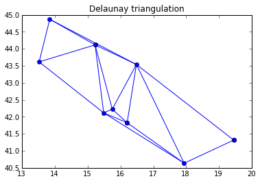
The Mare Adriaticum is our current test bed in Pleiades. We've made 9 different connections to it from precisely located islands, ports, and promontories. These play the part of the tagged photos in the Flickr story, and here they are as a GeoJSON feature collection: https://gist.github.com/3886076#file_mare_adriaticum_connections.json. My alpha shape analysis begins with a Delaunay triangulation of the space between these points. I used scipy.spatial.Delaunay to do it and benefited from the examples in this Stack Overflow post: http://stackoverflow.com/questions/6537657/python-scipy-delaunay-plotting-point-cloud.

import json
import numpy as np
from scipy.spatial import Delaunay

# JSON data from the gist above.
coordinates = [f['geometry']['coordinates'] for f in json.loads(data)]
points = np.array(coordinates)
tri = Delaunay(np.array(points))

# Rest as in SO post above.
...

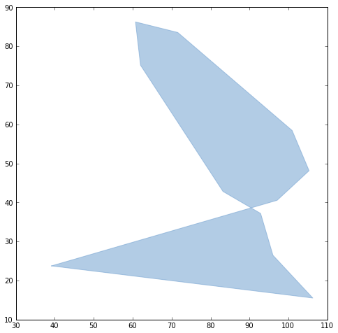
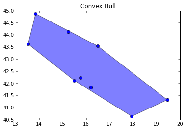
The nodes and lines of this triangulation are shown to the left below. Dissolving them yields the convex hull of the points, a figure that is slightly too big for Pleiades: points we want to have on the boundary of the Adriatic Sea, Iader to the north and the tip of the Gargano Promontory to the sourth, fall inside the hull. By what criteria might we toss out the peripheral triangles of which they are nodes and obtain an alpha shape more representative of the Adriatic? Printing out the radii of each triangle's circumcircle gives us this list:

0.916234205371
21.0145482369
1.85517410861
1.79158041604
0.887999941617
0.983745009567
1.2507779965
1.01471746864
0.430582735954
6.79200819757

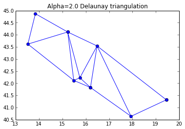
All of these are radii on the order of 1 except for 2 outliers. Those outliers are the narrow triangles we want to exclude from our hull. Setting a radius limit of 2 (α=0.5) via the code below removes the outlier triangles.

import math

edges = set()
edge_points = []
alpha = 0.5

# loop over triangles:
# ia, ib, ic = indices of corner points of the triangle
for ia, ib, ic in tri.vertices:
    pa = points[ia]
    pb = points[ib]
    pc = points[ic]

    # Lengths of sides of triangle
    a = math.sqrt((pa[0]-pb[0])**2 + (pa[1]-pb[1])**2)
    b = math.sqrt((pb[0]-pc[0])**2 + (pb[1]-pc[1])**2)
    c = math.sqrt((pc[0]-pa[0])**2 + (pc[1]-pa[1])**2)

    # Semiperimeter of triangle
    s = (a + b + c)/2.0

    # Area of triangle by Heron's formula
    area = math.sqrt(s*(s-a)*(s-b)*(s-c))

    circum_r = a*b*c/(4.0*area)

    # Here's the radius filter.
    if circum_r < 1.0/alpha:
        add_edge(ia, ib)
        add_edge(ib, ic)
        add_edge(ic, ia)

lines = LineCollection(edge_points)
plt.figure()
plt.title('Alpha=2.0 Delaunay triangulation')
plt.gca().add_collection(lines)
plt.plot(points[:,0], points[:,1], 'o', hold=1)

I dissolved the triangles using Shapely and render the hull using PolygonPatch from descartes.

from descartes import PolygonPatch
from shapely.geometry import MultiLineString
from shapely.ops import cascaded_union, polygonize

m = MultiLineString(edge_points)
triangles = list(polygonize(m))

plt.figure()
plt.title("Alpha=2.0 Hull")
plt.gca().add_patch(PolygonPatch(cascaded_union(triangles), alpha=0.5))
plt.gca().autoscale(tight=False)
plt.plot(points[:,0], points[:,1], 'o', hold=1)
plt.show()

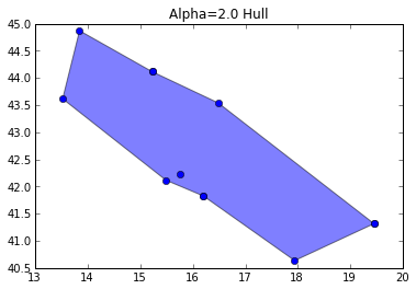
Can you see the difference? The hull pulls down a bit on the north edge and bumps up a bit on the south edge. It may not look like much to you, but now we're rescuing the Gargano Massif from the Adriatic – a fascinating place with unique geologic formations and 3 species of native giant hamsters. Who knows how many or how large these may have been in ancient times? (Update 2012-10-15: It's unlikely that Romans encountered the giant hamsters and hedgehogs of Pliocene Gargano.)

I've put a lot of work into making Shapely play well with Numpy and Matplotlib through the Python geospatial data protocol; it's fun to experiment with them like this. That interface also makes publishing a web map of my alpha shape trivial. The shape is exported to GeoJSON with a few lines of Python

from shapely.geometry import mapping

hull_layer = dict(
    type='FeatureCollection',
    features=[dict(
        type='Feature',
        id='1',
        title='Hull (Alpha=2.0)',
        description='See http://sgillies.net/blog/1154/the-fading-shape-of-alpha',
        geometry=mapping(cascaded_union(triangles)) )])

print json.dumps(hull_layer, indent=2)

and copied to a script in http://sgillies.github.com/mare-adriaticum to be used with Leaflet. Leaflet! If the new OpenLayers is designed around first-class treatment for GeoJSON we may yet return, but for now it's all Leaflet all the time in Pleiades.

I've run out of time today for playing with and writing about ancient alpha shapes, but have list of next things to do. It's obvious that I should be using the Web Mercator projection at least and probably an equal area projection when computing the circumcircles and triangulation and also obvious that there's no globally ideal alpha value. A statistical analysis of the circumcircle radii for each shape is certainly the right way to determine the outliers, and there may be different kinds of distributions involved. Meanwhile, this alpha shape of the Adriatic gets better as we anchor it to more precisely located places. A few more at the north end and the resulting shape has bounding box and centroid properties not much different than what you might come up with from an Adriatic Sea shape derived from a world coastlines dataset.

Enumeration of the problems I see in asserting fine boundaries for unmeasurable or intrinsically fuzzy places is another TODO item.

(With apologies to Aaron Straup Cope for the title of this post.)

I've written that I was going to do something about the lack of GeoRSS support in feedparser. JSON seems to have eclipsed Atom and RSS at the cutting edge of things, but XML syndication formats remain a sound, minimally-coupled way to integrate systems on the web. The feedparser is still important to me and I want to see it have first-class spatial support. Today I tracked down the official GitHub repo of the current maintainer, forked it, and patched my old diff in, tests and all. The results are here: https://github.com/sgillies/feedparser/tree/georss.

Below is a bit of code that builds on my previous example of making Robinson projection maps using Pyproj, matplotlib, and no for loops. There is a function to make circular buffers around feed entry locations with a radius proportional to earthquake magnitude and one to label the locations. Each of these functions are simplified by the GeoJSON style property attached to entries by my feedparser patch. The feed I'm using is one of the last hour's quakes from the USGS.

from shapely.geometry import mapping, shape

feed = feedparser.parse(
    "http://earthquake.usgs.gov/earthquakes/catalogs/1hour-M1.xml")

def quake(entry):
    # entries have a ``where`` item that provides the Python geospatial
    # interface and can be operated on by geospatial packages
    title = entry.get('title', "M 0.0,")
    m, val = title.split(",")[0].split(" ")
    radius = 1.0 + 4.0*float(val)
    patch = shape(entry['where']).buffer(radius)
    return {"title": title, "geometry": mapping(patch)}

def label(fig, entry):
    x, y = transform_robin(*entry['where']['coordinates'])
    fig.gca().text(x, y, entry['title'], fontsize='large')
    return fig

quakes = imap(quake, filter(lambda x: x.get('where'), feed.entries))
fig = reduce(
        partial(add_record, fc=RED, ec=RED, alpha=0.5),
        imap(robinson, quakes),
        fig )
fig = reduce(
        label,
        filter(lambda x: x.get('where'), feed.entries),
        fig )
fig.gca().set_title(feed['updated'])
fig.savefig("quake.png")

The result is below. The circular buffers are not circles in the Robinson projection.

With my feedparser patch, GeoRSS feed entries become simple to operate on with Shapely, descartes, PySAL, ArcPy, or other software that understands the GeoJSON-like Python geospatial interface: https://gist.github.com/2217756. Please, like-minded people, leave a favourable comment at https://github.com/kurtmckee/feedparser/pull/9.

Python 3.3 is out. I use buildout.python to configure and make pythons on OS X.

(p33)krusty-2:p33 seang$ python
Python 3.3.0 (default, Sep 29 2012, 10:03:39)
[GCC 4.0.1 (Apple Inc. build 5493)] on darwin
Type "help", "copyright", "credits" or "license" for more  information.
>>>

I'm continuing to have fun with functional style Python map hacking. I've blogged about different aspects of this, but here's my first try at putting it all together: data access to map projection to folding everything down into a map image. After writing three functions operating on single feature records (one for drawing, one for projection, one for weighting by attributes), I can get a basic choropleth map of world population density in 4 lines of Python. I'll introduce those functions one at a time starting with feature drawing.

Next, feature projection using Pyproj (and PROJ4).

Finally, classification of features by their attributes.

Code like zip(*func(*zip(*ring)) is probably taking it a little bit too far. While Python permits functional programming, its syntax isn't designed for readibility of functional code.

Update (2012-09-06): I've made 2 kinds of edits to the source in the gists. First, I've changed the drawing function so that it takes and returns a Matplotlib figure and noted why the function is impure. Mutability is essential to Matplotlib figures, there's no easy around this. The second bunch of edits restores as much referential transparency as I can: although the figures are mutable, they are only instantiated within the reduce expression and therefore can't be mutated by any other code.

It's been a while since I've used or written about Clojure, but I seized an opportunity to do so today. A Shapely user has been wondering what is up with simple, yet invalid polygons. The following WKT polygon:

"POLYGON ((0 0, 0 2, 2 2, 2 0, 0 0), (0 0, 0 1, 1 1, 1 0, 0 0))"

has a 2x2 square exterior ring and a square 1x1 interior ring that snaps precisely into its lower left quadrant.

The interior ring is not a true "hole" because the rings overlap. In the simple features sense this is an invalid polygon, and Shapely (with GEOS 3.3.0) confirms it.

>>> ring1 = [(0, 0), (0, 2), (2, 2), (2, 0), (0, 0)]
>>> ring2 = [(0, 0), (1, 0), (1, 1), (0, 1), (0, 0)]
>>> from shapely.geometry import Polygon
>>> q = Polygon(ring1, [ring2])
>>> q.area
3.0
>>> q.is_valid
False

But what's this?

>>> q.is_simple
True

GEOS is a port of JTS – what would JTS do? I'm not a Java programmer, but there's Clojure: its REPL is a handy means of answering that question. I've got JTS and JTSIO 1.8.0 in my classpath here.

user=> (def wkt
    "POLYGON ((0 0, 0 2, 2 2, 2 0, 0 0), (0 0, 0 1, 1 1, 1 0, 0 0))")
#'user/wkt
user=> wkt
"POLYGON ((0 0, 0 2, 2 2, 2 0, 0 0), (0 0, 0 1, 1 1, 1 0, 0 0))"
user=> (def p (.read (com.vividsolutions.jts.io.WKTReader.) wkt))
#'user/p
user=> p
#<Polygon POLYGON ((0 0, 0 2, 2 2, 2 0, 0 0), (0 0, 0 1, 1 1, 1 0, 0 0))>
user=> (.getArea p)
3.0
user=> (.isValid p)
false
user=> (.isSimple p)
true

JTS, too, says it's simple. Maybe simple features simplicity isn't meaningful for polygons... and a check of the JTS source confirms this.

[isSimple()] Returns true, since by definition LinearRings are always simple.

I can see the rationale, but I think we'll consider breaking with JTS and GEOS on this one. It would be a first.

Update (2012-09-02)

In hindsight, the case above isn't such a good example. The rings themselves are simple. The polygon is only invalid because they overlap. Instead, here's the case of a bowtie polygon with a self-crossing exterior ring and no interior rings.

wkt = ("POLYGON (("
       "39.1451330299999967 23.7510081600000014, "
       "97.0537220899999937 40.5455008799999987, "
       "105.2652701399999984 48.1330221300000005, "
       "100.9175268500000016 58.4333681499999997, "
       "71.5608144800000048 83.5511480100000057, "
       "60.7118916800000008 86.2531609899999978, "
       "62.0046980799999972 75.1478175999999962, "
       "83.1631000699999987 42.8207167300000009, "
       "92.8230586199999976 37.1917558199999974, "
       "95.9940112900000031 26.4705124599999984, "
       "106.2205448200000006 15.5197519199999991, "
       "39.1451330299999967 23.7510081600000014"
       "))" )

bowtie = loads(wkt)
reduce(draw, [bowtie], gca())

Note that I'm exploiting Python's implicit line joining and string literal concatenation to give a little bit of structure to this geometry's WKT representation.

The test of simplicity is performed by GEOS, in which the exterior ring and polygon are simple by defintion.

print bowtie.is_valid
print bowtie.is_simple
print bowtie.exterior.is_simple

False
True
True

If we test the ring as though it were a line we get the opposite result.

from shapely.geometry import LineString
print LineString(bowtie.exterior).is_simple
# False

Whether rings should be simple by definition is, I feel, more a matter of taste than correctness. Letting rings report that they are in fact not simple is more to my taste. The simplicity of a polygon would then be the product of the simplicity of its rings.

from itertools import chain
print all(r.is_simple for r in chain([bowtie.exterior], bowtie.interiors))
# True

By the way, Python's all() short circuits in a good way: as soon as is_simple evaluates to False in the chain, it returns False.

This is very sad news. I use John's Matplotlib often and blogged about it just yesterday. His close friends have set up a memorial fund to help ensure the education of his children.

Update (2012-08-31): I'm watching his recent SciPy keynote (via Kurt Schwehr).