Rasterio 0.6
I uploaded Rasterio 0.6 to PyPI today. The new features are tags (aka GDAL metadata) and colormaps.
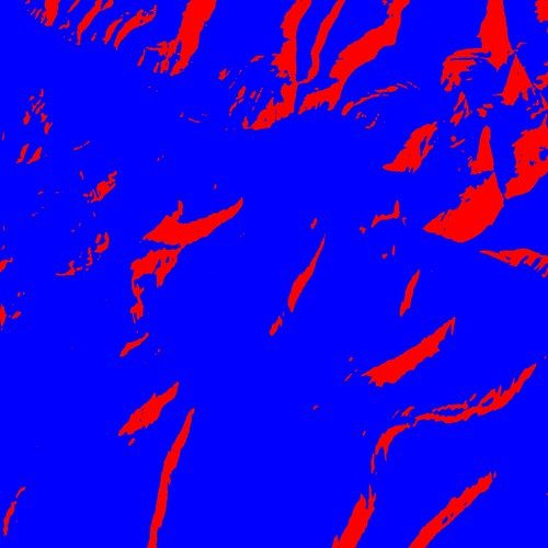
With just a couple lines of Python you can turn this simple greyscale image
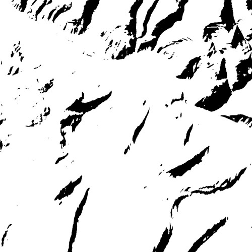
into an eye-searing RGB color image.
I uploaded Rasterio 0.6 to PyPI today. The new features are tags (aka GDAL metadata) and colormaps.
With just a couple lines of Python you can turn this simple greyscale image
into an eye-searing RGB color image.
I released Fiona 1.1.1 and rasterio 0.5.1 yesterday. There are a couple bug fixes, but the main features are the interactive data inspectors fiona.insp
$ fiona.insp docs/data/test_uk.shp
Fiona 1.1.1 Interactive Inspector (Python 2.7.5)
Type "src.schema", "next(src)", or "help(src)" for more information.
>>>
and rasterio.insp.
$ rasterio.insp rasterio/tests/data/RGB.byte.tif
Rasterio 0.5.1 Interactive Inspector (Python 2.7.5)
Type "src.name", "src.read_band(1)", or "help(src)" for more information.
>>>
I'm not sure why I didn't think of this before, but last night after the nth time launching python in interactive mode, importing rasterio, and typing in a filename with no tab completion, I made myself an interactive raster dataset inspector for Rasterio. Oh, and yes, I made it for you, too. Then I made one for Fiona.
You've used Python's interpreter interactively before, yes? By which I mean typing "python" at a shell prompt to get the banner and triple right-angle bracket prompt.
$ python
Python 2.7.5 (default, Oct  3 2013, 20:27:52)
[GCC 4.2.1 Compatible Apple LLVM 5.0 (clang-500.2.76)] on darwin
Type "help", "copyright", "credits" or "license" for more information.
>>>
I've used code.interact() to give you the same kind of prompt right after calling rasterio.open() on a filename you provide to the main function in rasterio.tool(). The code is ridiculously simple.
$ python -m rasterio.tool rasterio/tests/data/RGB.byte.tif
Rasterio 0.5.1 Interactive Interpreter
Type "src.name", "src.read_band(1)", or "help(src)" for more information.
>>>
Typing in the first two suggested expressions gives you useful entry points.
>>> src.name
'rasterio/tests/data/RGB.byte.tif'
>>> src.read_band(1)
array([[0, 0, 0, ..., 0, 0, 0],
       [0, 0, 0, ..., 0, 0, 0],
       [0, 0, 0, ..., 0, 0, 0],
       ...,
       [0, 0, 0, ..., 0, 0, 0],
       [0, 0, 0, ..., 0, 0, 0],
       [0, 0, 0, ..., 0, 0, 0]], dtype=uint8)
it's a bit like gdalinfo on steroids. You can get statistics by using Numpy ndarray methods, because rasterio has ndarrays instead of band objects.
>>> red = src.read_band(1)
>>> red.min(), red.max(), red.mean()
(0, 255, 29.94772668847656)
Fiona's inspector is in the fiona.inspector module.
$ python -m fiona.inspector docs/data/test_uk.shp
Fiona 1.1.1 Interactive Inspector
Type "src.name", "src.schema", "next(src)", or "help(src)" for more information.
>>>
Its suggested expressions give you (with the help of pprint.pprint()):
>>> src.name
u'test_uk'
>>> import pprint
>>> pprint.pprint(src.schema)
{'geometry': 'Polygon',
 'properties': OrderedDict([(u'CAT', 'float:16'), (u'FIPS_CNTRY', 'str'), (u'CNTRY_NAME', 'str'), (u'AREA', 'float:15.2'), (u'POP_CNTRY', 'float:15.2')])}
>>> pprint.pprint(next(src))
{'geometry': {'coordinates': [[(0.899167, 51.357216),
                               (0.885278, 51.35833),
                               (0.7875, 51.369438),
                               (0.781111, 51.370552),
                               (0.766111, 51.375832),
                               (0.759444, 51.380829),
                               (0.745278, 51.39444),
                               (0.740833, 51.400276),
                               (0.735, 51.408333),
                               (0.740556, 51.429718),
                               (0.748889, 51.443604),
                               (0.760278, 51.444717),
                               (0.791111, 51.439995),
                               (0.892222, 51.421387),
                               (0.904167, 51.418884),
                               (0.908889, 51.416939),
                               (0.930555, 51.398888),
                               (0.936667, 51.393608),
                               (0.943889, 51.384995),
                               (0.9475, 51.378609),
                               (0.947778, 51.374718),
                               (0.946944, 51.371109),
                               (0.9425, 51.369164),
                               (0.904722, 51.358055),
                               (0.899167, 51.357216)]],
              'type': 'Polygon'},
 'id': '0',
 'properties': OrderedDict([(u'CAT', 232.0), (u'FIPS_CNTRY', u'UK'), (u'CNTRY_NAME', u'United Kingdom'), (u'AREA', 244820.0), (u'POP_CNTRY', 60270708.0)]),
 'type': 'Feature'}
I'd like to have proper program names for these soon instead of "python -m rasterio.tool", but haven't thought of any yet. Also, I will gladly accept patches that would use your own favorite other interpreters (bpython, IPython) if available.
As it's getting more use at work, I've moved rasterio to Mapbox's GitHub organization and wrote about it on the Mapbox blog. Mapbox is probably known more for Javascript, but has a lot of Python programs running at any moment and more in development.
What do I mean when I write that rasterio is Python software, not GIS software? There is GIS software under the hood, obviously, and rasterio would be nowhere without the excellent GDAL library. What I mean is that whenever faced with a design choice between the way something would be done in a name brand GIS program and the way it would be done in Python, I always choose the Python way. That means I/O is done via file-like objects. That means no reliance on side effects. Python dicts instead of GIS-specific types or microformatted strings. It means embracing Python idioms and protocols. Making things iterable and zip-able. It means PEP 8 and PEP 20.
This is not to say that I think Python is the best language for every application or that Python language design is always right. I'm increasingly a polyglot and I expect that you are, too, or will be soon. It seems clear to me that one of the main keys to successful polyglot programming isn't using interfaces that stick to the common features of languages, it's using the best parts of various languages to their fullest. I believe this means idiomatic Javascript in your Javascript programs (for example) and idiomatic Python in your Python programs. Celebrating Python is what I'm doing to make rasterio a better tool for polyglots.
Bill Dollins recently wrote about some of the characteristics of GIS software, and here is the crux of it:
So I have come to realize that the mainstream GIS community has become very much like my professor’s theoretical cat; conditioned to take the long way to the end result when more direct paths are clearly available. What’s more, they have become conditioned to think of such approaches as normal.
Python, on the other hand, is supposed to be direct, highly productive, and fun. I've chosen to make rasterio less like the GIS software Bill wrote about and more like ElementTree, simplejson, Requests, pytest, and Numpy – packages that make the most of Python's strengths.
By the way, I wrote to the Python Software Foundation's Trademark Committee to make extra sure that my derived work (the GeoJSON file at https://gist.github.com/sgillies/8655640#file-python-powered-json) was legit, and received a very clear and friendly response from David Mertz in the affirmative. I've been a reader of his articles for years and it was a pleasure to correspond with him at last. Python isn't just a great language, it's great people.
$ pip install 'rasterio>=0.5'
Which is to say, share and enjoy.
Here's a script that shows off everything new in rasterio 0.5: GDAL driver environments, raster feature sieving, and a generator of raster feature shapes.
#!/usr/bin/env python
#
# sieve: demonstrate sieving and polygonizing of raster features.

import subprocess

import numpy
import rasterio
from rasterio.features import sieve, shapes

# Register GDAL and OGR drivers.
with rasterio.drivers():

    # Read a raster to be sieved.
    with rasterio.open('rasterio/tests/data/shade.tif') as src:
        shade = src.read_band(1)

    # Print the number of shapes in the source raster.
    print "Slope shapes: %d" % len(list(shapes(shade)))

    # Sieve out features 13 pixels or smaller.
    sieved = sieve(shade, 13)

    # Print the number of shapes in the sieved raster.
    print "Sieved (13) shapes: %d" % len(list(shapes(sieved)))

    # Write out the sieved raster.
    with rasterio.open('example-sieved.tif', 'w', **src.meta) as dst:
        dst.write_band(1, sieved)

# Dump out gdalinfo's report card and open (or "eog") the TIFF.
print subprocess.check_output(
    ['gdalinfo', '-stats', 'example-sieved.tif'])
subprocess.call(['open', 'example-sieved.tif'])
The images that you can operate on with the new functions in rasterio.features don't have to be read from GeoTIFFs or other image files. They could be purely numpy-based spatial models or slices of multidimensional image data arrays produced with scipy.ndimage.
For fun and benchmarking purposes I've written a program that uses both Fiona and rasterio to emulate GDAL's gdal_polygonize.py: rasterio_polygonize.py. If you're interested in integrating these modules, it's a good starting point.
JSON-LD, a a JSON-based serialization for Linked Data, is finally a W3C Recommendation. I'd like to remind readers that dumpgj, the any-vectors-to-GeoJSON program that is distributed with Fiona, will optionally add JSON-LD contexts to GeoJSON files.
$ dumpgj --help
usage: dumpgj [-h] [-d] [-n N] [--compact] [--encoding ENC]
              [--record-buffered] [--ignore-errors] [--use-ld-context]
              [--add-ld-context-item TERM=URI]
              infile [outfile]

Serialize a file's records or description to GeoJSON

positional arguments:
  infile                input file name
  outfile               output file name, defaults to stdout if omitted

optional arguments:
  -h, --help            show this help message and exit
  -d, --description     serialize file's data description (schema) only
  -n N, --indent N      indentation level in N number of chars
  --compact             use compact separators (',', ':')
  --encoding ENC        Specify encoding of the input file
  --record-buffered     Economical buffering of writes at record, not
                        collection (default), level
  --ignore-errors       log errors but do not stop serialization
  --use-ld-context      add a JSON-LD context to JSON output
  --add-ld-context-item TERM=URI
                        map a term to a URI and add it to the output's JSON LD
                        context
In a C program using the GDAL (or OGR) API, you manage the global format driver registry like gdalinfo does:
#include "gdal.h"

int main( int argc, char ** argv )
{

    /* Register all drivers. */
    GDALAllRegister();

    ...

    /* De-register all drivers. */
    GDALDestroyDriverManager();

    exit( 1 );
}
I used to try to hide this in Python bindings by calling GDALAllRegister() in a module and registering a function that called GDALDestroyDriverManager() with the atexit module.
""" gdal.py """

import atexit

def cleanup():
    GDALDestroyDriverManager()

atexit.register(cleanup)

GDALAllRegister()
Importing that gdal module registers all drivers and the drivers are de-registered when the module is torn down. I don't like this approach anymore. I prefer that driver registration to not be a side effect of module import. And in testing, I'm finding that it's a drag to write the code needed to keep the cleanup function around until the atexit handlers execute.
Instead of going back to the C style, I'm going to go forward with context managers and a with statement to manage the GDAL and OGR global driver registries. The with rasterio.drivers() expression creates a GDAL driver environment.
import rasterio

try:

    # Use a with statement and context manager to register all the
    # GDAL/OGR drivers.
    with rasterio.drivers():

        # Count the manager's registered drivers (156 in this case).
        print rasterio.driver_count()

        # Open a file and get to work.
        with rasterio.open('rasterio/tests/data/RGB.byte.tif') as f:

            # Oops, an exception.
            raise Exception("Oops")

        # When this block ends, even via an exception, the drivers are
        # de-registered.

except Exception, e:
    print "Caught exception: %s" % e

# Drivers were de-registered and this will print 0.
print rasterio.driver_count()

# Output:
# 156
# Caught exception: Oops
# 0
The nice thing about this approach is that the registered drivers get de-registered and the memory deallocated no matter what happens in the with block. And it's less code than my old approach using atexit.
So that programs written for older versions of Fiona and rasterio don't break, I'm also letting opened collections and datasets manage the driver registry if no other manager is already present. So this code below works as before.
import rasterio

try:

    with rasterio.open('rasterio/tests/data/RGB.byte.tif') as f:
        print rasterio.driver_count()
        raise Exception("Oops")

except Exception, e:
    print "Caught exception: %s" % e

print rasterio.driver_count()

# Output:
# 156
# Caught exception: Oops
# 0
It's more efficient to register drivers once and only once in your program, so use with fiona.drivers() or with rasterio.drivers() in new programs using Fiona 1.1 and rasterio 0.5 or newer.
I've just added a new function to rasterio that generates the shapes of all features in an image. The region labeling algorithm is provided by libgdal's GDALPolygonize() and I'm using GDAL and OGR in-memory raster and vector datastores to avoid disk I/O. Look, Ma, no temporary files.
In the interpreter session shown below, I made a 12 x 12 image with three different features: the background with value 1, a 4 x 4 square in the upper left corner with value 2, and a 2 x 2 square with value 5 on the left edge. Then I copied an affine transformation matrix from the rasterio test suite and passed it and the image to rasterio.features.shapes(). The result: the polygon boundaries of those three features in "world", not image, coordinates.
>>> import pprint
>>> import numpy
>>> from rasterio import features
>>> image = numpy.ones((12, 12), dtype=numpy.uint8)
>>> image[0:4,0:4] = 2
>>> image[4:6,0:2] = 5
>>> image
array([[2, 2, 2, 2, 1, 1, 1, 1, 1, 1, 1, 1],
       [2, 2, 2, 2, 1, 1, 1, 1, 1, 1, 1, 1],
       [2, 2, 2, 2, 1, 1, 1, 1, 1, 1, 1, 1],
       [2, 2, 2, 2, 1, 1, 1, 1, 1, 1, 1, 1],
       [5, 5, 1, 1, 1, 1, 1, 1, 1, 1, 1, 1],
       [5, 5, 1, 1, 1, 1, 1, 1, 1, 1, 1, 1],
       [1, 1, 1, 1, 1, 1, 1, 1, 1, 1, 1, 1],
       [1, 1, 1, 1, 1, 1, 1, 1, 1, 1, 1, 1],
       [1, 1, 1, 1, 1, 1, 1, 1, 1, 1, 1, 1],
       [1, 1, 1, 1, 1, 1, 1, 1, 1, 1, 1, 1],
       [1, 1, 1, 1, 1, 1, 1, 1, 1, 1, 1, 1],
       [1, 1, 1, 1, 1, 1, 1, 1, 1, 1, 1, 1]], dtype=uint8)
>>> t = [101985.0, 300.0379266750948, 0.0,
...      2826915.0, 0.0, -300.041782729805]
>>> for shape, value in features.shapes(image, transform=t):
...     print("Image value:")
...     print(value)
...     print("Geometry:")
...     pprint.pprint(shape)
...
Image value:
2
Geometry:
{'coordinates': [[(101985.0, 2826915.0),
                  (101985.0, 2825714.832869081),
                  (103185.15170670037, 2825714.832869081),
                  (103185.15170670037, 2826915.0),
                  (101985.0, 2826915.0)]],
 'type': 'Polygon'}
Image value:
5
Geometry:
{'coordinates': [[(101985.0, 2825714.832869081),
                  (101985.0, 2825114.7493036212),
                  (102585.0758533502, 2825114.7493036212),
                  (102585.0758533502, 2825714.832869081),
                  (101985.0, 2825714.832869081)]],
 'type': 'Polygon'}
Image value:
1
Geometry:
{'coordinates': [[(103185.15170670037, 2826915.0),
                  (103185.15170670037, 2825714.832869081),
                  (102885.11378002529, 2825714.832869081),
                  (102585.0758533502, 2825714.832869081),
                  (102585.0758533502, 2825114.7493036212),
                  (102285.0379266751, 2825114.7493036212),
                  (101985.0, 2825114.7493036212),
                  (101985.0, 2823314.4986072425),
                  (105285.41719342604, 2823314.4986072425),
                  (105585.45512010113, 2823314.4986072425),
                  (105585.45512010113, 2826915.0),
                  (103185.15170670037, 2826915.0)]],
 'type': 'Polygon'}
In its initial form, the function generated GeoJSON-ish feature dicts, but I decided these were too heavy and have switched to a pair of objects: one a GeoJSON style geometry dict and the other the labeled feature's characteristic image value.
This example doesn't read or write because I want to show how the new function doesn't require I/O. But of course you can always get the numpy array and affine transformation matrix from a raster on disk using rasterio.open() and read_band(), and the generated shapes can be written to a vector file on disk using fiona.open() and writerecords().
I got some feedback about yesterdays blog post. To be clear, I'm not suggesting that multipart geometry types are not needed. Rather, I think it's the single part types that may be superfluous.
A couple of you suggest that single points and sets of points are different from the higher dimensional (curve and surface) cases. What exactly sets these geometry types apart and is the argument for setting them apart a geometrical one? Consider the two WKT strings below and the geometric point sets they describe.
POINT(0 0)
MULTIPOINT((0 0))
You're banking on the distances from either of these objects to any other object, or a 50-meter buffer zone around either object, being the same. In a Simple Features world, you're also counting on these objects being equal (See section 2.1.13.3, Named Spatial Relationship predicates based on the DE-9IM, in OGC 99-049). Applications using Shapely, to name one category of users, are certainly banking on it.
>>> from shapely.geometry import Point, MultiPoint
>>> coords = (0.0, 0.0)
>>> Point(coords).equals(MultiPoint([coords]))
True
If a single point with coordinates x,y is equivalent to a set of points with a single member (same coordinates x,y), why do we trouble ourselves with different representations for these things? I'm sure historical reasons are a big part of the answer. Not just "Feature B followed Feature A" historical reasons, but point-in-time historical reasons. I've a half-baked thesis that the late 90s and early 00s are partly characterized by information modeling practices that tended to produce the greatest possible number of classes rather than the least sufficient number of classes.
Just thinking out loud here. And GeoJSON is the context for my thinking: how it came to be and how things might have been done differently. And how things might be done differently the next time around.
Sometimes I agree with Martin Daly's suggestion that the Shapefile was right all along. Not about everything, of course, but about the lack of distinction between the geometric objects that the OGC's Simple Features model classifies as polygons and multipolygons. What's the essential difference between a polygon and a set of non-intersecting polygons with only one member? I'm not convinced that there is one. Consider the features in the image below (from http://education.usgs.gov/kids/tracks.html).
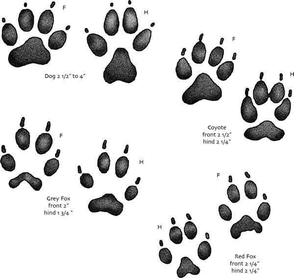
In the simple features model, you'd classify all of these nine-part prints as multipolygon features. In the coyote's hind print, however, the slight merger of the middle toe prints hints at what we might see if the prints were made in a soft enough medium: single part contiguous prints.
Why would we want the representation in data of a print to change from a multi-part multipolygon to a single polygon as we dilate it (by making it deeper in this analogy)? If I was designing a format for the exchange of animal print data, I'd like all prints to be of the same geometric type whether they were shallow or deep. Wouldn't you? If not, why not? What would be the use of having separate polygon and multi-polygon types and prints that flip-flop between them depending on incidental conditions of their observation? And would any use outweigh the cost of documenting and explaining the difference?